Isoquant Curve

What is Isoquant Curve?

Isoquant Curve: A technical relation that shows how inputs are converted into output is depicted by an isoquant curve. It shows the optimum combinations of factor inputs with the help of prices of factor inputs and their quantities that are used to produce the same output.

The term ISO implies equal and quant means quantity or output.

For example, for producing 100 calendars, 90 units of capital and 10 units of labour are used.

Isoquant curves are also called as equal product curves or production indifference curves.

Table of Content [Show]

Isoquant Curve Definition

An isoquant is a curve showing all possible combinations of inputs physically capable of producing a given level of output.Ferguson

An isoquant curve may be defined as a curve showing the possible combinations of two variable factors that can be used to produce the same total product.Peterson

Assumptions of Isoquant Curve

The assumptions of an isoquant curve are as follows:

There are only two factor inputs, labour and capital, to produce a particular product.
Capital, labour and goods are divisible in nature.
Capital and labour are able to substitute each other up to a certain limit.
Technology of production is given over a period of time.
Factors of production are used with full efficiency.

Let us learn isoquant with the help of the following table.

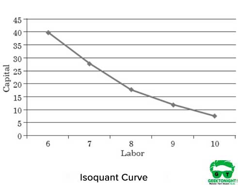
Table 1 shows the different combinations of two factor inputs, namely, labour and capital for producing 150 tonnes of output:

LABOUR	CAPITAL
6	40
7	28
8	18
9	12
10	8

Table 1: Combinations of Two Factor Inputs

Figure 1 shows the isoquant curve of different labour capital combinations that help in producing 150 tonnes of output:

Properties of Isoquant Curve

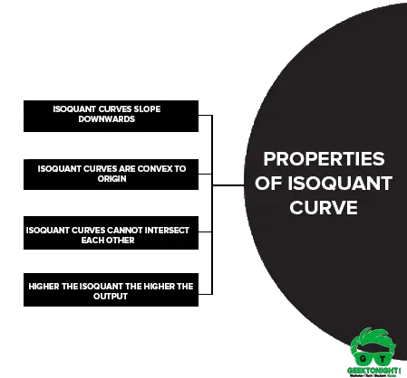
Some of the properties of isoquant curve are as follows:

Isoquant curves slope downwards

It implies that the slope of the isoquant curve is negative. This is because when capital (K) is increased, the quantity of labour (L) is reduced or vice versa, to keep the same level of output.

Isoquant curves are convex to origin

It implies that factor inputs are not perfect substitutes. This property shows the substitution of inputs and diminishing marginal rate of technical substitution of isoquant. The marginal significance of one input (capital) in terms of another input (labour) diminishes along with the isoquant curve.

Figure 2 shows the convex isoquant curve:

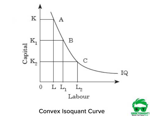
The convexity represents that the MRTS diminishes if we move from point A to B and from B to C along the isoquant. The MRTS diminishes because the two inputs labour and capital are not perfect substitutes.

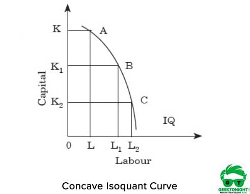
Thus, for every increase in labour, there is a decrease in capital. If isoquant is concave, the MRTS of labour for capital increases. Figure 3 shows the concave isoquant curve:

As shown in Figure 3, if we move from point A to B and from B to C along the isoquant, the MRTS increases. It shows that the two inputs labour and capital are perfect substitutes. Thus, for every increase in labour, there is an increase in capital.

Isoquant curves cannot intersect each other

An isoquant implies the different levels of combination producing different levels of inputs. If the isoquants intersect each other, it would imply that a single input combination can produce two levels of output, which is not possible. The law of production would fail to be applicable.

Higher the isoquant the higher the output

It implies that the higher isoquant represents higher output. The upper curve of the isoquant produces more output than the curve beneath. This is because the larger combination of input results in a larger output as compared to the curve that is beneath it.

Marginal Rate of Technical Substitution

The slope of the isoquant curve is the rate of substitution that shows how one input can be substituted for another while holding the output constant. This is called marginal rate of technical substitution (MRTS).

According to Lipsey, “the marginal rate of technical substitution may be defined as the rate at which one factor is substituted for another with output held constant.”

The formula for calculating MRTS is as follows:
MRTS = – ∆K/∆L
where, ∆K = Change in capital
∆L= Change in labour

The formula shows that at a given level of output, MRTS of capital for labour would imply the amount of labour that the firm would be willing to give up for an additional unit of capital. Similarly, MRTS of labour for capital would imply the amount of capital that the firm would be willing to give up for an additional unit of labour.

MRTS is also equal to the ratio of marginal product of one input to the marginal product of another input. The output along the isoquant is constant. If the change in labour is substituted for the change in capital, then the increase in output due to increase in labour should match with the decrease in output due to decrease in capital. Mathematically

∆L x MP_L= ∆K x MP_k
∆Q= ∆L x MP_L + ∆K x MP_k

Since the output remains unchanged at a given isoquant,

∆L x MP_L + ∆K x MP_k = 0

(MP_L / MP_K)= (- ∆K / ∆L)

MRTS_KL = (MP_L / MP_K)

Thus, we can say that MRTS between inputs is equal to marginal products of the inputs.

The MRTS is calculated as shown in Table 2

LABOUR	CAPITAL	MRTS
6	40
7	28	12:1
8	18	10:1
9	12	6:1
10	8	4:1

Table 2: MRTS

Types of Isoquant Curve

There is a continuous substitution of one input variable by the other input variable at a diminishing rate. Perfect complements and perfect substitutes give different forms of isoquants.

The different types of isoquant curve are as follows:

Linear isoquant

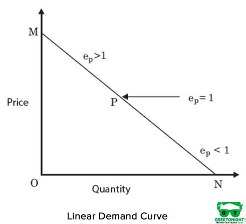
It is a straight line isoquant and represents a perfect substitutability between the inputs, capital and labour of the production function. MRTS between inputs remains constant. Figure 4 shows a linear isoquant:

The algebraic form of production function in case of linear isoquant is as follows:

Q = aK + BL

Here, Q is the weighted sum of K and L. The slope of the curve can be calculated with the help of following formula:

MP_K = ∆Q/∆K = a
MP_L = ∆Q/∆L = b
MRTS = MP_L / MP_K
MRTS = -b/a (b/a is constant)

However, linear isoquant does not have existence in the real world.

L-shaped isoquant

This is the case of perfect complements. Under this, the combination between capital and labour is in a fixed proportion. Only one combination of labour and capital is possible to produce a product with affixed proportion of inputs.

For increasing the production, an organisation needs to increase both inputs proportionately. The graphical representation of fixed factor proportion isoquant is L in shape, shown in Figure 5:

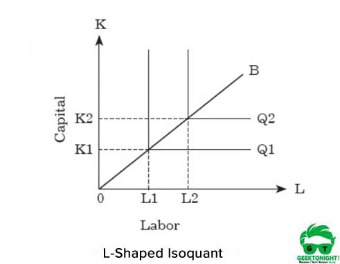
As shown in Figure 5, the L-shaped isoquant represents that there is no substitution between labour and capital and they are assumed to be complementary goods. It can be seen that OK1 units of capital and OL1 units of labour are required for the production of Q1.

On the other hand, to increase the production from Q1 to Q2, an organisation needs to increase inputs from K1 to K2 and L1 to L2 both. This relationship between capital and labour can be expressed as follows:

Q = f (K, L) = min (aK, bL)

where, min implies Q equals to lower of the two terms, aK and bL

For example, in case aK > bL, then Q = bL and in case aK < bL then, Q = aK.

This isoquant is same as leontif production function.

Elasticity of Substitution Between Factors

We know that MRTS is the slope of the isoquant. However, it does not reveal the degree of substitutability of one factor to another. It is important to measure the degree of substitutability between the two inputs.

Therefore, economists have developed a formula for estimating the extent of substitutability between the two inputs, capital and labour, which is known as elasticity of factor substitution.

Elasticity of factor substitution (σ) refers to the ratio of percentage change in capital-labour ratio to the percentage change in MRTS.

It is mathematically represented as follows:

σ = percentage change in capital labour ratio/percentage change in MRTS

Or,

σ = [(∆K/∆L) /∆MRTS] * [MRTS/ (K/L)]

If ∆K/∆L = ∆MRTS ; σ = 1
If ∆K/∆L > ∆MRTS ; σ > 1
If ∆K/∆L < ∆MRTS ; σ < 1

High elasticity of substitution between factors implies that the factors can easily be substituted to each other, while a low elasticity represents that substitution of factors is possible to a certain extent.

In case of linear isoquant, the substitution elasticity would be infinite, and in case of L-shaped isoquants, it would be zero.

ISO Cost Curves

Iso-cost curve is the locus of points of all different combinations of labour and capital that an organisation can employ, given the price of these inputs. Iso-cost line represents the price of factors along with the amount of money an organisation is willing to spend on factors.

In other words, it shows different combinations of factors that can be purchased at a certain amount of money. The slope of the iso-cost line depends upon the ratio of price of labour to the price of capital.

For example, a producer has a total budget of ₹120, which he wants to spend on the factors of production, namely, X and Y. The price of X in the market is ₹15 per unit and the price of Y is ₹10 per unit. Table 7.5 depicts the combinations:

COMBINATIONS	UNITS OF X	UNITS OF Y	TOTAL EXPENDITURE
A	8	0	120
B	6	3	120
C	4	6	120
D	2	9	120
E	0	12	120

The iso-cost line is shown in Figure 7.8:

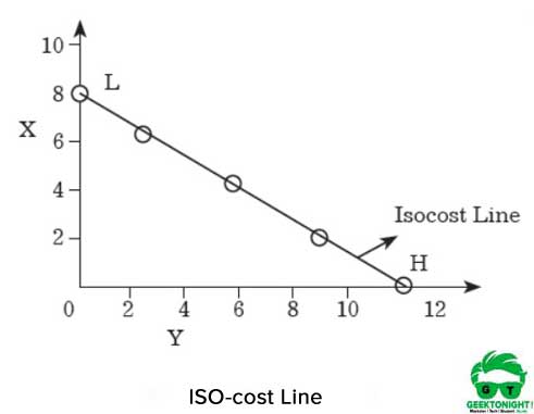
As shown in Figure 6, if the producer spends the whole amount of money to purchase X, then he/she can purchase 8 units of X. On the other hand, if the producer purchases Y with the whole amount, then he/she would be able to get 12 units.

If points H and L are joined on X and Y axes, respectively, then a straight line is obtained, which is called iso-cost line. All the combinations of X and Y that lie on this line, would have the same amount of cost that is ₹120.

Similarly, other iso-cost lines can be plotted by taking cost more than 120, in case the producer is willing to spend more amount of money on the production factors.

With the help of isoquant and iso-cost lines, a producer can determine the point at which inputs yield maximum profit by incurring minimum cost. Such a point is termed as producer’s equilibrium.