What is Indifference Curve

What is Indifference Curve?

Indifference curve can be defined as the locus of points each representing a different combination of two good, which yield the same level of utility and satisfaction to a consumer.

Indifference Curve definition, properties, assumptions, significance, criticism

Table of Content [Show]

Therefore, the consumer is indifferent to any combination of two commodities if he/she has to make a choice between them. This is because an individual consumes a variety of goods over time and realises that one good can be substituted with another without compromising on the satisfaction level.

When these combinations are plotted on the graph, the resulting curve is called indifference curve. This curve is also called the iso-utility curve or equal utility curve.

Definitions of Indifference Curves

Different economists have defined indifference curves in different ways. Some of these definitions are given below:

Prof. Henderson and Prof. Quandt have defined, “The locus of all commodity combinations from which a consumer derives the same level of satisfaction forms an indifference curve.”

Prof. A.L. Mayers has defined, “An indifference schedule may be defined as a schedule of various combinations of goods that will be equally satisfactory to the individual concerned. If we depict this in the form of a curve, we get an indifference curve.”

According to Edgeworth, “Indifference curve is that path on which a substitution on a particular commodity by another in any manner or quantity gives the consumer the same satisfaction in any position.”

According to Prof. J.M. Joshi, “An indifference curve is a locus of points which are geometrical representations of a combination of commodities (x and y) such that the consumer is indifferent among any of these combinations.”

Prof. J.K. Smith has defined, “It is a locus of the points representing pairs of quantities between which the individual is indifferent, so it is termed as indifference curve.”

Indifference Curve Analysis

Let us learn the indifference curve through a schedule. Assume that a consumer consumes two commodities X and Y and makes five combinations for the two commodities a, b, c, d, and e, which is shown in Table 1:

COMBINATION	UNITS OF COMMODITY Y	UNITS OF COMMODITY X	TOTAL UTILITY
a	25	3	U
b	15	5	U
c	8	9	U
d	4	17	U
e	2	30	U

Table 1: Indifference Schedule For Substitutes X and Y

When the indifference schedule for X and Y is plotted on a graph, a curve is obtained, which is shown in Figure 1.

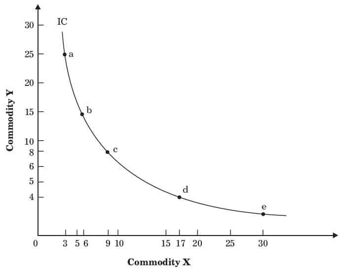
On the indifference curve (IC), there can be several other points in between the points a, b, c, d, and e, which would yield the same level of satisfaction to the consumer. Therefore, the consumer remains indifferent towards any combinations of two substitutes yielding the same level of satisfaction.

Indifference Curve Properties

The indifference curve (IC) has certain definite properties or characteristics, which are as follows:

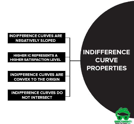
Indifference Curve Properties are:

Indifference Curves are negatively sloped

The indifference curves are sloped downwards to the right. The reason for the negative slope is that as a consumer increases the consumption of commodity X, he/ she sacrifices some units of commodity Y in order to maintain the same level of satisfaction.

Higher IC represents a higher satisfaction level

A higher IC lying above and to the right of another IC implies a higher level of satisfaction and vice versa. In simple words, the combination of commodities on the higher IC is preferred by a consumer to the combination that lies on a lower IC.

Indifference Curves are convex to the origin

ICs are curved inwards; thus they are convex to the origin. This implies that as the consumer continues to substitute commodity X for commodity Y, MRS of X for Y diminishes along the IC.

Indifference Curves do not intersect

This can be explained by considering a hypothetical situation where two indifference curves intersect. The point of intersection would then imply that a combination of commodities on the higher curve would offer the same level of satisfaction as that on the lower indifference curve, which violates the basic assumption of ICs.

Assumptions of Indifference Curve

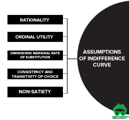
Assumptions of Indifference Curve are:

Rationality
Ordinal Utility
Diminishing Marginal Rate of Substitution
Consistency and Transitivity of Choice
Non-Satiety

Rationality

We have assumed our consumer a rational consumer he always aims at getting the maximum satisfaction (utility) out of his income taking the prices and other relevant information into account.

Ordinal Utility

The consumer ranks his preference according to the satisfaction of each combination. He does not know actually his satisfaction but he always expresses his preferences for the various bundles of commodities. Hence ordinal utility measurement is necessary and not cardinal measurement.

Diminishing Marginal Rate of Substitution

Indifference curves are assumed to be convex to the origin. It denotes that indifference curve technique is based on the axiom of diminishing marginal rate of substitution.

Consistency and Transitivity of Choice

It is assumed that the consumer’s behavior is consistent over the period. It means if a consumer, 1ooses combination A over combination B, at a given time, he will not choose combination B over combination A at some other time provided both the combinations are available to him.

Non-Satiety

It is assumed in the analysis that a consumer always prefers a large number of a good to smaller amount of that good provided that the amount of other goods at his disposal remains unchanged. It implies that the consumer never reaches at satiety point. This assumption is known as non-satiety assumption.

Application of Indifference Curve

The technique of indifference curves has assumed special significance because of its application in almost every sphere of economic activity. A few such applications can be mentioned as follows:

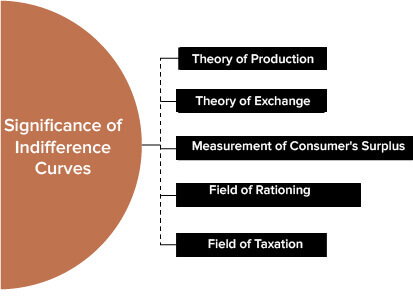
Application of Indifference Curve are:

Theory of Production

In the Theory of Production: The basic aim of a producer is to attain a low-cost combination. Indifference curves are useful in the realization of this objective. When we use these curves in the theory of production, they are called iso-product curves.

Theory of Exchange

In the Theory of Exchange: Prof. Edgeworth used the technique of indifference curves to show the mutual gains from the exchange of two goods between two consumers. Exchange makes 11, possible for both the consumers to reach a higher level of satisfaction.

Field of Rationing

In the field of Rationing: This technique can also be mad use of in the field of rationing. Ordinarily two commodities are rationed out to different individuals, irrespective of their preferences. But if their respective preferences are considered and the amounts of the two commodities be distributed among consumers in accordance with their scale of preferences, each of them shall be in a position to reach a higher indifference curve and satisfaction.

Measurement of Consumer Surplus

In the measurement of Consumer’s Surplus: Indifference curve technique has rehabilitated the old Marshallian concept of consumer’s surplus that has lain buried almost for decades under the weight of unrealistic and illusory assumptions. Consumer’s surplus can be measured with the help of this technique without any need for making unrealistic assumptions.

Field of Taxation

In the field of Taxation: The technique is also applied to test preference between a direct and indirect tax. With the help of indifference curves it can be shown that a direct tax is preferable to an indirect tax as regards its effects on consumption and satisfaction of the taxpayer.

Criticism of Indifference Curve

Although the concept of IC is vital to explain the ordinal approach, it is criticised on various grounds.

The main points of criticism of indifference curve are given below:

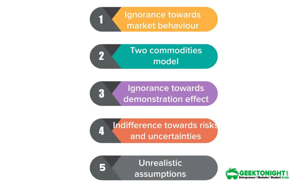
Let us discuss these points of of Indifference curve in detail:

Ignorance towards market behaviour

IC analysis considers only two commodities in the market. However, the market is full of a large number of commodities. Thus, it does not consider market behaviour in the analysis of consumer behaviour.

For example, a change in the price of other commodities in the market may affect the purchase of the commodities being considered.

Two commodities model

IC analysis is based on the combinations of two commodities. Considering more than two commodities in IC analysis makes the calculations more complex. This may further make it difficult to predict consumer behaviour.

Ignorance towards demonstration effect

The demonstration effect states that an individual’s consumption pattern is affected by the level of consumption of other individuals. This is ignored by IC analysis limiting its use to understand consumer behaviour.

Indifference towards risks and uncertainties

Risks and uncertainties in the market and individual’s life are inevitable.

Unrealistic assumptions

IC is based on an assumption that a consumer is fully aware of his/her preference for various commodities. However, this is an unrealistic assumption as humans have their limitations.

What is Indifference Curve