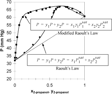
In Section 10.7 we demonstrated that deviations from Raoult’s law were manifested by changes in the bubble line and thus characterized positive and negative deviations. With a purely mathematical perspective for modeling the behavior, we could develop a “correction” to Raoult’s law as illustrated in Fig 11.1.

Figure 11.1. P-x-y diagram for isopropanol water at 30°C illustrating the rationale for activity coefficients using modified Raoult’s law. Data from Udovenko, V.V., and Mazanko, T.F. 1967. Zh. Fiz. Khim. 41:1615.
Note that the bubble line for Raoult’s law misses the shape completely. The bubble pressure formula for Raoult’s law is linear in x1 because x2 = 1 – x1 and the Psat values are constants with respect to x1. Suppose that we were to apply a “correction” to VLE K-ratio for each component and attribute the deviations to the liquid phase, where the molecules are closely packed and molecular geometry and intermolecular potentials are much more important than in the vapor phase. The resultant method provides

The relation to the bubble line is not yet obvious. Cross-multiplying and summing gives,

Now we can begin to see how this approach adjusts the model to the bubble pressure. When a system has positive deviations from Raoult’s law, the bubble line lies above the Raoult’s law bubble line ![]() , therefore γi > 1. When a system has negative deviations, γi < 1. This correction factor γi, is referred to as the activity coefficient. Therefore, P-x-y data are related to the deviations of the activity coefficients from unity, or it may be helpful to consider the sign of ln γi.1 Look back at Fig. 11.1 and the figures in Section 10.7 and note that the deviations from Raoult’s law disappear as pure compositions are approached. This means that the deviations depend on composition, and that the γi(x) that we have introduced in Eqn. 11.1 must go to 1 as the solution becomes pure in the ith component.
, therefore γi > 1. When a system has negative deviations, γi < 1. This correction factor γi, is referred to as the activity coefficient. Therefore, P-x-y data are related to the deviations of the activity coefficients from unity, or it may be helpful to consider the sign of ln γi.1 Look back at Fig. 11.1 and the figures in Section 10.7 and note that the deviations from Raoult’s law disappear as pure compositions are approached. This means that the deviations depend on composition, and that the γi(x) that we have introduced in Eqn. 11.1 must go to 1 as the solution becomes pure in the ith component.
As you might imagine, there are rules that we should follow to develop feasible functions. We discuss those theoretical aspects in the upcoming sections. The accepted method of modeling the system is to build a model for γi(x) based in the excess Gibbs energy. The excess Gibbs energy is also discussed in upcoming sections, but briefly it is the Gibbs energy in “excess” of an ideal solution. It is generally positive when γi > 1 and negative when γi < 1. The model for excess Gibbs energy can be developed from a theoretical model of mixing behavior, and usually contains adjustable parameters to adjust the magnitude and skewness of the “excess” and thus fit the experiment.
Activity coefficients may be determined from experimental measurements by rearranging modified Raoult’s law as implied by Eqn. 11.1:

From the values of the activity coefficients, a value for excess Gibbs energy can be calculated:

These values may be tabulated to provide GE/RT vs. x1 and the resultant curve can be regressed to fit a reasonable analytical expression for convenient interpolation at all compositions. Empirically, it is often preferable to fit the γi’s directly. We demonstrate both approaches.
The three major stages of working with activity coefficients are shown in Fig. 11.2. In Stage I, the activity coefficients are determined at various compositions from the experiments. In Stage II, a model is selected and various techniques can be used to fit the model to the experimental data. Finally, in Stage III, the model is utilized to solve many different types of phase equilibria problems. Initially, we work some examples where Stage II is separate from Stage III. In advanced fitting, Stages II and III are combined. In addition to development of these skills, much of the chapter is devoted to demonstrating the theoretical foundations for the models so that you are familiar with some of the popular models available in process design software. We integrate examples of bubble, dew, and flash calculations throughout the discussions.

Figure 11.2. Strategy for using excess Gibbs energy models for activity coefficients. Experiments are used to determine γi in Stage I. A model is selected and the model is fitted in Stage II. The model is utilized to extend and extrapolate the experimental results in Stage III.
The One-Parameter Margules Equation
The simplest expression for the Gibbs excess function is the one-parameter Margules equation (also known as the two-suffix Margules equation). For a binary system,

![]() The one-parameter Margules equation is the simplest excess Gibbs expression.
The one-parameter Margules equation is the simplest excess Gibbs expression.
Note: The parameter A12 is a constant which is not associated with the other uses of the variable (equation of state parameters, Helmholtz energy, Antoine coefficients) in the text. The parameter A12 is typically used in discussions of the Margules equation, so we use it here.2
The one-parameter Margules equation is symmetrical with composition. It has an extremum at x1 = 0.5 in a binary system and becomes zero at purity of either component. The activity coefficients in a binary system for the one-parameter Margules equation are (derived later as Eqns. 11.29–11.31),

![]() Margules one-parameter model for a binary mixture.
Margules one-parameter model for a binary mixture.
Let us fit the model to experimental data to demonstrate Stage I and Stage II procedures.
Example 11.1. Gibbs excess energy for system 2-propanol + water
Using data from the 2-propanol(1) + water(2) system presented in Fig. 10.8 calculate the excess Gibbs energy at x1 = 0.6369 and fit the one-parameter Margules equation. Data from the original citation provide T = 30°C, ![]() ,
, ![]() , and y1 = 0.6462 when x1 = 0.6369 at P = 66.9 mmHg.
, and y1 = 0.6462 when x1 = 0.6369 at P = 66.9 mmHg.
Solution
The approach is to determine the activity coefficients and then relate them to the excess Gibbs energy. The Stage I step is


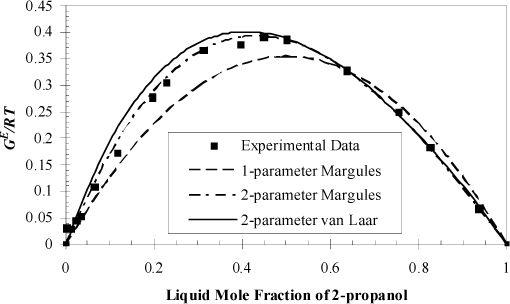
If we were given more experimental data, we could repeat the calculation for each data point, thus creating a plot of GE versus x1 like the points shown in Fig. 11.3.

Figure 11.3. Illustration of calculation of GE from experiment and fitting of Margules models to a single point as discussed in Examples 11.1 and 11.5, for 2-propanol + water, with the experimental data points from Fig. 10.8 on page 395. Data are tabulated in Example 11.8. The van Laar model fit to a single point is explained in Section 12.2.
Then, we have been instructed to use the one-parameter Margules model for Stage II. Let us fit the model as given by Eqn. 11.5 and using the value from Eqn. 11.7.

The curve of GE versus x1 is shown in Fig. 11.3 along with the two-parameter models to be discussed in Section 11.6 and Example 11.5.
Note from the example that the single point fit gives only an approximate representation of the excess Gibbs energy (because we compared to some additional data that were not included in the problem statement). However, let us proceed to see how this one data point can be leveraged to study the phase behavior.
Leave a Reply