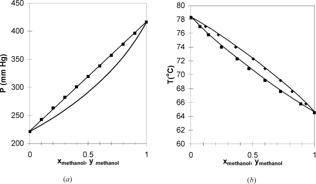
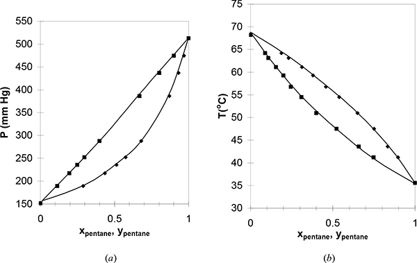
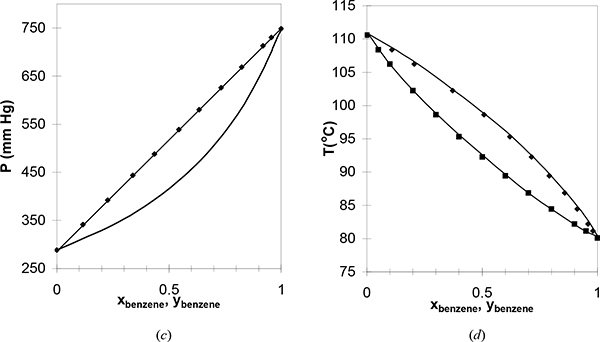
For a small class of mixtures where the components have very similar molecular functionality and molecular size, the bubble-pressure line is found to be a linear function of composition as shown in Figs. 10.2 and 10.3. As was noted in Section 10.1, the T-x-y and P-x-y diagram shapes are related qualitatively by inverting one of the diagrams. Because the bubble pressure is a linear function of composition, we may write for a binary system,


Figure 10.2. (a), (b). Phase behavior of the methanol-ethanol system. Left figure at 50°C. Right figure at 760 mm Hg. (P-x-y from Schmidt, G.C. 1926. Z. Phys. Chem. 121:221, T-x-y from Wilson, A., Simons, E.L. 1952. Ind. Eng. Chem. 44:2214).

Figure 10.3. (a), (b) Phase behavior of the pentane-hexane system. Left figure at 25°C. Right figure at 750 mm Hg. (P-x-y from Chen, S.S., Zwolinski, B.J. 1974. J. Chem. Soc. Faraday Trans. 70: 1133, T-x-y from Tenn, F.G., Missen, R.W. 1963. Can. J. Chem. Eng. 41:12).

Figure 10.3. (c); (d) Phase behavior of the benzene-toluene system. Left figure at 79.7°C. Right figure at 760 mm Hg. (P-x-y from Rosanoff, M.A., et al. 1914. J. Am. Chem. Soc. 36:1993, T-x-y from Delzenne, A.O. 1958. Ind. Eng. Chem., Chem. Eng. Data Series. 3:224).
![]() Raoult’s Law for Bubble Pressure.
Raoult’s Law for Bubble Pressure.
Dividing by P, we find the form of the bubble objective function summarized in Table 10.1,

Therefore, we conclude that the K-ratio for Raoult’s law4 is

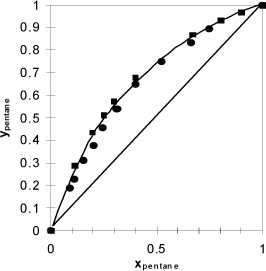
Throughout Chapters 10–16 and 18–19 we continually improve and refer to K-value models. The motivation for this focus on K-values is that they are used for all types of separations. For this select class of mixtures, the K-ratios depend only on T and P and are independent of composition. To calculate a K-ratio, we can use any method for the vapor pressure. Though we have derived the K-ratio empirically, we use this model to practice performing VLE calculations and return in future sections to a more fundamental derivation to explore more fully the restrictions for this model. In future chapters, we explore more sophisticated methods for estimating the K-ratio when Raoult’s law does not apply and the K-ratios depend on composition. In addition to the P-x-y and T-x-y plots, another common presentation of data for distillation studies is the x-y plot of coexisting compositions as shown in Fig. 10.4.

Figure 10.4. Data from Fig. 10.3 plotted with coexisting liquid and vapor values for each experimental tie line, resulting in the x-y plot. Note that the data do not superimpose exactly because one data set is isobaric and the other set is isothermal. Squares are T-x-y data. Circles are P-x-y data. The diagonal is traditionally drawn in an x-y figure, and the data never cross the diagonal for systems that follow Raoult’s law.
![]() K-values are used for all types of separations.
K-values are used for all types of separations.
François-Marie Raoult (1830–1901) was a French chemist who studied freezing point depression and the effect of mixing on bubble pressure. His first work on solution behavior in 1878 dealt with freezing point depression. His paper on “Raoult’s Law” was published in 1892.
Shortcut Estimation of VLE K-ratios
Given Raoult’s law and recalling the Chapter 9 shortcut procedure for estimating vapor pressures, it is very useful to consider combining these to give a simple and quick method for estimating ideal solution K-ratios. Substituting, we obtain the shortcut K-ratio,

Since the ideal solution model is somewhat crude anyway, it is not unreasonable to apply the above equation as a first approximation for any ideal solution when rapid approximations are needed.5
![]() Shortcut K-ratio for Raoult’s law. Not only is this expression restricted to Raoult’s law, but it is also subject to the restrictions of Eqn. 9.11.
Shortcut K-ratio for Raoult’s law. Not only is this expression restricted to Raoult’s law, but it is also subject to the restrictions of Eqn. 9.11.
Bubble Pressure
For a bubble-pressure calculation, writing ![]() as
as ![]() , which is
, which is  . Multiplying by P, we may write

![]() Note that as we begin applications, some of the equations are model-dependent.
Note that as we begin applications, some of the equations are model-dependent.
where no iterations are required because temperature, and therefore vapor pressures, are known. Once the bubble pressure is found, the value can be reinserted into Eqn. 10.6 to find the vapor mole fractions:

Dew Pressure
For a dew-pressure calculation, writing ![]() as
as ![]() and rearranging:
and rearranging:

which may be rearranged and solved without iteration, because the vapor pressures are fixed at the specified temperature:

Once the dew pressure is calculated, the value can be reinserted into Eqn. 10.6 to find the liquid mole fractions:

Bubble Temperature
For a bubble-temperature calculation, writing ![]() as
as ![]() , and rearranging:
, and rearranging:

To solve this equation, it is necessary to iterate on temperature (which changes Pisat) until P equals the specified pressure. Then the vapor phase mole fractions are calculated using Eqn. 10.9.
Dew Temperature
For a dew-temperature calculation, writing ![]() as
as ![]() , and rearranging:
, and rearranging:

To solve this equation, it is necessary to iterate on temperature (which changes Pisat) until P equals the specified pressure. Then the liquid phase mole fractions are calculated using Eqn. 10.12.
General Flash
Flash drums are frequently used in chemical processes. For an isothermal drum, the temperature and pressure of the drum are known. Consider that a feed stream is liquid which becomes partially vaporized after entering the drum as illustrated in Fig. 10.5. The name of the flash procedure implies that it is applicable only for flashing liquids, but in fact, the procedure is also valid for vapor entering a partial condenser or for any number of incoming vapor and/or liquid streams with overall compositions specified by {zi} with overall flow rate F. To apply the procedure, the overall composition of the components, zi, total feed flow rate, F, and outlet T and P just need to be known before the procedure is started. Though the method is introduced using flowing streams, flow is not required for a flash calculation; the calculation can be performed for any overall composition constrained at a particular temperature and pressure even within a closed system. Also, the inlet stream temperature does not need to match the outlet temperature; the two outlet streams are at the specified temperature.

Figure 10.5. Illustration of a flash drum and variable definitions for streams. Note that F need not be a liquid; F may be all vapor or partial vapor. The principles can be applied to a nonflowing system as described for a binary on page 371.
The flash equations are easily derived by modification of the overall and component balances used in the development of the lever rule in Section 10.1. If z is the feed composition and V/F is the liquid-to-feed ratio, then L/F = 1 – V/F, and the component balance is zi = xi(L/F) + yi(V/F). Substituting for L/F from the overall balance, and using yi = xiKi, the component balance becomes zi = xi[(1 – V/F) + Ki(V/F)], which can be solved for xi:

using yi = xiKi, we may multiply Eqn. 10.15 by Ki to obtain yi.

One obvious thing to do at this point is to iterate to find the V/F ratio which satisfies ![]() . But the flash problem is different from the dew- and bubble-point problems because we must also solve
. But the flash problem is different from the dew- and bubble-point problems because we must also solve ![]() . Fortunately, a reliable successive substitution method has been developed by Rachford and Rice6 to solve this problem using the objective function
. Fortunately, a reliable successive substitution method has been developed by Rachford and Rice6 to solve this problem using the objective function ![]() . Introducing the variable Di ≡ xi – yi to denote the difference between xi and yi for each component,
. Introducing the variable Di ≡ xi – yi to denote the difference between xi and yi for each component, ![]() , we iterate on V/F until the sum approaches zero. For a binary system, using the Ki ratios, the objective function becomes
, we iterate on V/F until the sum approaches zero. For a binary system, using the Ki ratios, the objective function becomes

For Raoult’s law, Ki is a function of temperature and pressure only, both of which are fixed for an general flash calculation. The outlets are assumed to exit at phase equilibrium, and the exit conditions are used to calculate Ki. Therefore, in Eqn. 10.17, the only unknown is V/F. Eqn. 10.17 is monotonic in V/F; the sum always increases as V/F increases. Therefore, we search for the value of V/F which satisfies the equation. Note that 0 < V/F < 1 for a physically realistic answer. Outside this range, the system is either below the dew pressure (mathematically V/F > 1) or above the bubble pressure (mathematically V/F < 0). After finding V/F from our basis, then, L/F = 1 – V/F and stream compositions can be found from Eqns. 10.15 and 10.16.
Before executing a flash calculation by hand, bubble and dew calculations at the overall composition are recommended to ensures that the flash drum is between the bubble and dew pressures at the given temperature. (These calculations are easier than the flash calculation and may save you from doing it if the system is outside the phase envelope.) When using a computer, the value of V/F can be used to ascertain if the system is outside the two-phase region. If a computer flash calculation does not converge, then the bubble or dew should be performed to troubleshoot.
For a binary system, a flash calculation may be avoided by plotting the overall composition on the P-x-y diagram between the dew and bubble pressures and reading the vapor and liquid compositions from the graph. Application of the lever rule permits calculation of the total fraction that is vapor; however, this method requires a lot of calculations to generate the diagram if it is not already available and is limited to binary mixtures. Also, plotting the curves is slower than a direct calculation.
The steady-state energy balance for an general flash is given by

where we indicate a common method of calculation of the enthalpy of a mixture as the sum of the component enthalpies and the heat of mixing (Eqn. 3.24 on page 105). Writing in terms of V/F:

A reference state must be specified for each component, and a method for calculation of the enthalpy must be selected. A simple method of calculating enthalpies of vapors and liquids relative to reference states has been illustrated in Example 3.3 on page 107. For an isothermal flash, the VLE constraint, Eqn. 10.17, can be solved independently of the energy balance, and the energy balance can then be solved for the required heat transfer.
Adiabatic Flash
An adiabatic flash differs from an isothermal flash because ![]() in Eqn. 10.19. The adiabatic conditions will result in a temperature change from the feed conditions that is often significant. A typical scenario involves an outlet pressure less than the inlet pressure, resulting in an evaporation of a fraction of the feed. Because evaporation is endothermic, this type of flash results in a temperature drop (often significant). We have seen this type of calculation for pure fluids using throttles in Chapter 5. The additional complication with a mixture is that the components will distribute based on their different volatilities. The objective of an adiabatic flash calculation is to determine the outlet temperature in addition to the L and V compositions. An adiabatic flash requires that Eqn. 10.19,
in Eqn. 10.19. The adiabatic conditions will result in a temperature change from the feed conditions that is often significant. A typical scenario involves an outlet pressure less than the inlet pressure, resulting in an evaporation of a fraction of the feed. Because evaporation is endothermic, this type of flash results in a temperature drop (often significant). We have seen this type of calculation for pure fluids using throttles in Chapter 5. The additional complication with a mixture is that the components will distribute based on their different volatilities. The objective of an adiabatic flash calculation is to determine the outlet temperature in addition to the L and V compositions. An adiabatic flash requires that Eqn. 10.19, ![]() , must be solved simultaneously with Eqn. 10.17. The vapor and liquid mole fractions for Eqn. 10.19 are determined from Eqns. 10.15 and 10.16. The method is complex enough that even simple assumptions, such as ideal mixing (ΔHmix = 0), benefit from a computer algorithm.
, must be solved simultaneously with Eqn. 10.17. The vapor and liquid mole fractions for Eqn. 10.19 are determined from Eqns. 10.15 and 10.16. The method is complex enough that even simple assumptions, such as ideal mixing (ΔHmix = 0), benefit from a computer algorithm.
The algorithm to solve for the adiabatic flash depends on the differences in boiling points of the components. Usually the boiling points are different enough that an initial guess of T is used in VLE Eqn. 10.17 (where V and L are assumed to exit at the same T) to find an initial V/F where 0 < V/F < 1. With that initial V/F, then the V and L compositions (Eqns. 10.15 and 10.16) and then the energy balance (Eqn. 10.19) are evaluated, often scaling Eqn. 10.19 by dividing by 1000 when the enthalpy values are large. If the energy balance is not satisfied, then a new T trial is inserted into Eqn. 10.17 and the loop continues. Eqn. 10.19 is monotonic in T and increases when T decreases. When the boiling points are very close for all components, such as with isomers, the calculation converges better with an initial guess of V/F in Eqn. 10.17, which is solved by trial and error for the T which satisfies the equation. The L and V compositions and T are then used for the outlet enthalpies in Eqn. 10.19 to generate a new value for V/F and the iteration continues until convergence.
Leave a Reply