What is Consumption Function

The functional relationship between consumption and national income is known as Consumption Function. It was introduced by John Maynard Keynes and represents the willingness of households to purchase goods and services at a given income level during a given period of time. It is represented as C = f(Y); where C = Consumption, Y = National Income and f = Functional Relationship. The consumption function is a psychological concept that shows consumption levels at different income levels in an economy. Besides, it is influenced by subjective factors like consumer habits, preferences, etc.

Consumption Function is based on the Psychological Law of Consumption introduced by Keynes. The Psychological Law of Consumption states three main things:

Even at zero income level, there is minimum consumption, i.e., autonomous consumption which is required for the survival needs of people.
Consumption increases with the increase in income.
The rate at which income increases is more than the rate of increase in consumption.

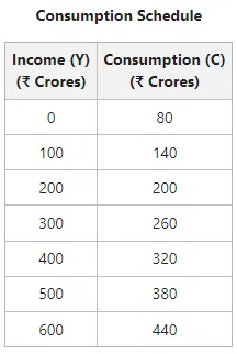
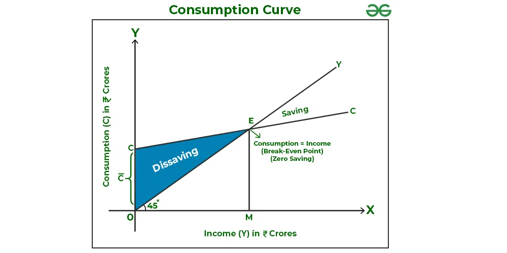
Let’s understand the concept of Consumption Function with the help of the following consumption schedule and consumption curve.

The above schedule shows consumption at different income levels.

In the above graph, X-axis represents National Income, and Y-axis represents Consumption Expenditure.

Observation:

1. Starting Point: The consumption curve (CC) starts from point C and not from point O, which means that even at a zero level of national income, there is autonomous consumption $(\bar{c})$ of OC.

2. Slope of Consumption Curve: The slope of the consumption curve CC is positive, which means that with an increase in income, consumption also increases. However, the rate at which consumption increases is less than the rate of increase in income because the consumer saves a part of his income and spends the rest.

3. Income is less than Consumption: As seen in the above table and graph, income is less than consumption at income levels less than ₹200 Crores and OM, respectively. This gap between consumption and income level is covered by dissavings. Dissavings is the previous savings of the consumer. In the above graph, dissavings is the shaded area $\Delta{COE}$ .

4. Break-even Point; i.e., C = Y: Break-even point is the point at which consumption is equal to income. In the above graph, the break-even point is achieved at point E with OM income level; i.e., at the income of ₹200 Crores. Also, at the break-even point, savings is zero.

5. Income is more than Consumption: As seen in the above table and graph, income is more than consumption at income levels more than ₹200 Crores and the points to the right of Point E, respectively. This excess income results in savings. It means that the gap after point E between the 45° line and the CC line represents positive savings.

Note: The 45° line is drawn to indicate whether the consumption is less than, equal to, or more than the income level.

Consumption is not the same as Consumption Function

Consumption is the amount of income spent on the purchase of goods and services at a given income level. However, Consumption Function is the schedule which shows the consumption expenditures at different income levels.

Types of Propensities to Consume

The two types of Propensities to Consume are Average Propensity to Consume (APC) and Marginal Propensity to Consume (MPC).

1. Average Propensity to Consume (APC):

It is the ratio of consumption expenditure to the corresponding income level. The formula to determine Average Propensity to Consume (APC) is:

Average~Propensity~to~Consume~(APC)=\frac{Consumption~(C)}{Income~(Y)}

APC can be equal to one, less than one, and more than one, but can never be zero. According to the formula, APC can be zero when the consumption level is zero, which is not possible at any income level because even at zero income level, there is autonomous consumption $(\bar{c})$ .

2. Marginal Propensity to Consume (MPC):

It is the ratio of the change in consumption expenditure to the change in total income. In simple terms, MPC explains the proportion of change income that is spent on consumption. The formula to determine Marginal Propensity to Consume (MPC) is as follows:

Marginal~Propensity~to~Consume~(MPC)=\frac{Change~in~Consumption~(\Delta{C})}{Change~in~Income~(\Delta{Y})}

The value of MPC varies between 0 and 1. Besides, the Marginal Propensity to Consume (MPC) of the poor is more than the MPC of the rich. It is because the poor spend most of their increased income on consumption as most of their basic needs are not yet fulfilled. However, rich people spend less of their increased income on consumption as they are already enjoying a high living standard.

Equation of Consumption Function

The consumption function consists of two parts:

Even at zero level of national income (Y), there is some minimum consumption; i.e., autonomous consumption $(\bar{c})$ . Autonomous consumption is always positive.
With an increase in income, the consumption level also increases. But the rate at which the consumption level increases is less than the rate of increase in income. The Marginal propensity to Consume (MPC) or b shows how the consumption expenditure (C) changes when there is a change in income. This part of consumption is Induced Consumption, and is equal to MPC x Income; i.e., b(Y).

Hence, the equation of Consumption Function will be:

Where,

C = Consumption

$(\bar{c})$ = Autonomous Consumption

b = MPC

Y = Income

In the above equation, a change in income does not have any impact on autonomous consumption expenditure; however, it affects the induced consumption expenditure. Also, as the given equation is a straight line with intercept $(\bar{c})$ and slope ‘b’, it is a case of the linear consumption function. Therefore, a higher value of b will result in a more slope of the linear consumption function.

The equation of the consumption function can be used to prepare the consumption curve by calculating consumption expenditure at different income levels if the value of (\bar{c}) ; i.e., autonomous consumption and b; i.e., MPS is given. For example, If the value of (\bar{c}) and b are ₹50 Crores and 0.80, respectively, then the Saving Expenditure at income level ₹100 crores will be

C = 50 + 0.80(100)

= 50 + 80

= ₹130 Crores