Plotting Ternary LLE Data

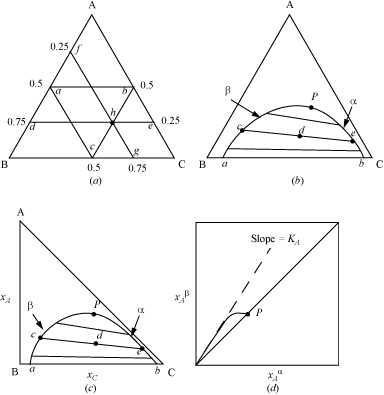
Graphical representation of ternary LLE data is important for design of separation processes. For ternary systems, triangular coordinates simultaneously represent all three mole fractions, or alternatively, all three weight fractions. Triangular coordinates are shown in Fig. 14.6(a), with a few grid lines displayed. The fraction of component A is represented by lines parallel to the BC axis: Along , the composition is x_A = 0.25; along , the composition is x_A = 0.5. The fraction of B is represented by lines parallel to the AC axis; along , the composition is x_B = 0.5; along , the composition is x_B = 0.25. The fraction of C is along lines parallel to the AB axis; along , x_C = 0.5. Combining these conventions, at point h, x_A = 0.25, x_B = 0.25, x_C = 0.5. An example of plotted LLE phase behavior is shown on triangular coordinates in Fig. 14.6(b). The compositions of coexisting α and β phases are plotted and connected with tie lines. The lever rule can be applied. For example, in Fig. 14.6(b), a feed of overall composition d will split into two phases: (moles β)/(moles α) = , and (moles β)/(moles feed) = .

Figure 14.6. Illustrations of graphical representation of ternary data on triangular diagrams. (a) Illustration of grid lines on an equilateral triangle; (b) illustration of LLE on an equilateral triangle; (c) illustration of LLE on a right triangle; (d) illustration of tie-line data on a right triangle.

To specify the composition of an arbitrary phase α in a ternary system, only two mole fractions are required. Since the mole fractions must sum to unity, if  and  are known, then the third mole fraction can be found, . The subscripts may be interchanged, and the same constraints hold for phase β. Therefore, cartesian coordinates can be used to plot two mole (or weight) fractions of each phase. Fig. 14.6(c) presents the data from Fig. 14.6(b) on cartesian coordinates. The tie line and lever rule concepts also apply on this diagram. Tie line data can be plotted on cartesian coordinates as in Fig. 14.6(d). This representation of tie line data permits improved accuracy when interpolating between experimental tie lines. The slope of the tie line data, as presented in Fig. 14.6(d), is frequently linear near the origin; the slope of the line in this region is , which is the distribution coefficient, K_i. For the LLE phase behavior shown in Fig. 14.6, the B + C miscibility is increased by the addition of A. Along the phase boundary, the tie lines become shorter upon approach to point P, the Plait point. Note that at the Plait point, all distribution coefficients are one.

Other Examples of LLE Behavior

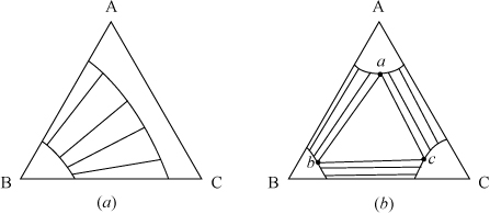
The ternary LLE of Fig. 14.6 is one of several common types. In this example, A + C is totally miscible (there is no immiscibility on the AC axis), as is A + B. When two of the three pairs of components are immiscible, the type of Fig. 14.7(a) can result, and when all three pairs have immiscibility regions, then type of Fig. 14.7(b) can result. In Fig. 14.7(b), the center region is LLL; since the T and P are fixed, any overall composition in the center triangle will split into the three phases of compositions a, b, and c, because F = C – P + 2 = 3 – 3 + 2 = 2.

Figure 14.7. Illustration of other types of LLE behavior.