Determination of intrinsic kinetics forms an essential and important component of chemical engineering kinetics. Typically, such determinations are carried out by bench-scale batch experiments wherein the concentrations of species are monitored as a function of time and the concentration-time data are subjected to analysis. Example 9.2.1 illustrates such analysis conducted for the determination of rate expression.
EXAMPLE 9.2.1 DETERMINATION OF RATE CONSTANT
A laboratory experiment is conducted to determine the rate constants for a reaction 2A → R. It is known that the reaction is second order with respect to A. The experiment involved measuring the concentration of the reactant A as a function of time in a batch vessel. The following is the data obtained. What is the value of the rate constant for the reaction?

Solution
The concentration-time relationship for a second-order reaction follows [3]:

Here, k2 is the rate constant for a second-order reaction having the units of (concentration · time)−1, L/mol h in this case.
As indicated by equation E9.1, the inverse of the concentration of A varies linearly with time. A graph of 1/CA versus t will have the rate constant k2 as its slope and 1/CA0 as the intercept. The rate constant can thus be obtained by a linear regression between 1/CA and t.
Solution (using Excel)
The solution steps using Excel are as follows:
1. Enter the raw data in the spreadsheet: time values in cells A3 through A11 and the concentration values in cells B3 through B11.
2. Calculate the inverse of concentration in cell B3 into cell C3 by entering the formula =1/B3. Copy the formula into cells C4 through C11 to calculate 1/CA.
3. Select the data in cells A3 through A11 and C3 through C11 by highlighting these cells: cells A3 through A11 are selected using the mouse, and then C3 through C11 are selected while pressing the Ctrl key to skip column B.
4. Create a graph by selecting Insert from the command menu bar, and then the X-Y scatter plot from the dropdown menu or by using the appropriate buttons. This plots data in cells C3 through C11 (1/CA) as a function of data in cells A3 through A11 (t).
5. Add various chart elements (axes titles, chart title) using the Design tab.
6. Insert a linear regression line by right-clicking on the data points, which opens a dialog box. Clicking the appropriate button inserts the regression line equation and correlation coefficient on the chart, as shown in Figure 9.4.
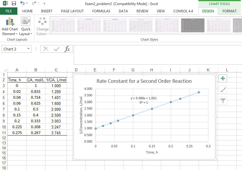
Figure 9.4 Excel solution to example 9.2.1.
Solution (using Mathcad)
The Mathcad solution is shown in Figure 9.5.
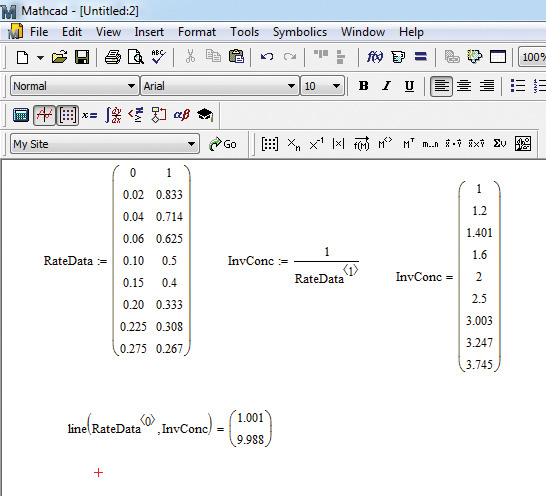
Figure 9.5 Mathcad solution to example 9.2.1.
The solution steps are as follows:
1. Enter the data in a matrix named RateData by first typing RateData: and then clicking on the matrix button. This opens a dialog box in which the number of rows (9) and columns (2) are entered, and the dialog box is closed by clicking OK. Enter the data with the first column having time values and the second column the concentration values.
2. Calculate the inverse of concentration values entered in the second column of RateData by typing InvConc:1/RateData<Ctrl+6> and then entering 1 in the placeholder. (The key combination <Ctrl+6> creates an index for the columns in variable RateData. The indices start from 0 for the first column, 1 for the second column, and so on.) The inverse values can be seen by typing InvConc=.
3. Use the line function to perform linear regression between the time (first column of RateData) and inverse concentration (InvConc). The line function has two arguments: the first one is the independent variable (the first column of RateData in this case), and the second is the dependent variable (InvConc). The keystrokes in this case are line(RateData<Ctrl+6>[space],InvConc), and then enter 0 in the index of RateData. Typing = after the closing parenthesis yields the solution consisting of a vector with two elements. The top number represents the intercept, and the bottom number represents the slope.
As can be seen from the figure, the rate constant value is 9.988 L/mol h, the same value obtained using Excel.
The material balance equation is sufficient for the design and analysis of a CSTR/MFR when heat effects need not be taken into account. However, an energy balance equation is also required when the heat effects are significant and need to be considered. For a given reactor volume, the material balance and the energy balance yield two different equations containing the conversion and the temperature, and these equations need to be solved simultaneously. Example 9.2.2 deals with this situation and existence of multiple solutions for an adiabatic operation of a CSTR.
EXAMPLE 9.2.2 CONVERSION IN A CSTR
The material balance and energy balance for a CSTR for a first-order reaction are given by equations E9.2 and E9.3, respectively [3]. What is the conversion in the reactor? What is its operating temperature?


Here, CPA is the mean specific heat capacity of the reactor contents. ![]() is the mean residence time of the material in the reactor—that is, the time it spends in the reactor—obtained by dividing the reactor volume by the volumetric flow rate (V/v). T0 is the inlet temperature (temperature of the feed stream). XEB and XMB are the conversions using the energy balance and the material balance on the reactor, respectively. ΔHrxn is the heat of reaction.
is the mean residence time of the material in the reactor—that is, the time it spends in the reactor—obtained by dividing the reactor volume by the volumetric flow rate (V/v). T0 is the inlet temperature (temperature of the feed stream). XEB and XMB are the conversions using the energy balance and the material balance on the reactor, respectively. ΔHrxn is the heat of reaction.
The data for the reactor are as follows:
T0 = 293 K, CPA = 810 J/mol K, ΔHrxn = −200 kJ/mol, V = 10 L, v = 0.2 L/s
A = 1.8 × 10⁵ s−1, Ea = 50 kJ/mol
Solution (using Mathcad)
The first step in the solution using Mathcad is plotting both XEB and XMB as functions of the temperature T. The values of the variables are specified first, followed by specifications of the range of the variable T, and the definitions of the two conversions. Both these functions are plotted against T using the Mathcad Graph utility. Figure 9.6 shows the plots generated.
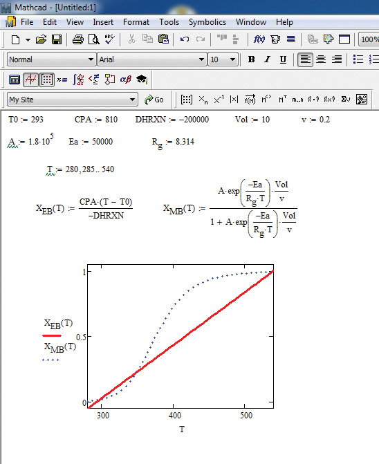
Figure 9.6 Conversions in the CSTR as a function of temperature.
As can be seen from the figure, the two curves intersect in three locations, implying that there are three possible solutions that satisfy the two equations. Examination of the three points reveals a very low, an intermediate, and a very high conversion. Since the objective is typically to convert as much of the reactant to the product as possible, the very high conversion is the desired operating point. The exact solution for conversion and temperature is obtained using the solve block in Mathcad, as shown in Figure 9.7.
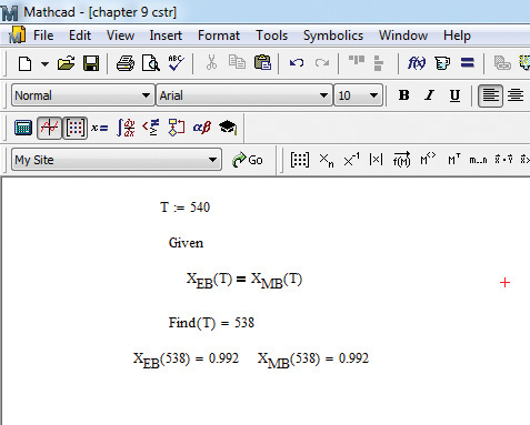
Figure 9.7 Exact solution at the high conversion point.
The procedure consists of providing an initial guess for temperature (540), specifying the objective function (equality of conversions), and then letting the program find the value of T that satisfies the objective function. As can be seen from the figure, the conversion will be 0.992 at the reactor temperature of 538 K, meaning that 99.2% of the reactant fed to the reactor will be converted to the desired product.
Figure 9.6, with its multiple intersection points for the energy balance and material balance conversion-time functions, indicates that multiple steady-state points are feasible while operating a CSTR. How the conditions are manipulated to operate at a particular point forms an interesting discussion in the course on chemical engineering kinetics.
Most of the reacting systems encountered in practice exhibit a much higher level of complexity than a simple first-order reaction. The desired reaction is invariably accompanied by an undesirable side reaction, which has significant impact on the economics of the process and increases the complexity of separations postreaction. These undesirable reactions include a parallel reaction that the reactant undergoes (A → S, when A → R is desired) or a series reaction (A → R → S, which reduces the amount of desired product R due to its consumption in the second reaction). Example 9.2.3 illustrates a computational problem related to a series reaction system.
EXAMPLE 9.2.3 CONVERSION AND SELECTIVITY IN A SERIES REACTION SYSTEM
Isopropenyl allyl ether isomerizes into allyl acetone according a first-order reaction with a rate constant given by k1 = 5.4 × 10¹¹ exp (−123000/RgT) s−1. Allyl acetone undergoes a first-order decomposition reaction having a rate constant of k2 = 4.9 × 10¹¹ exp (−131000/RgT) s−1, where the activation energies are expressed in J/mol. The rate constant equations reflect the Arrhenius dependence on temperature, with the universal gas constant denoted by the symbol Rg to distinguish it from the desired product R. The isomerization reaction is carried out in a PFR, with the desired CR,max/CA0 ratio of 0.8 in the product. What is the operating temperature of the reactor, assuming that the reaction is conducted isothermally? What is the conversion of A?
The relevant equations are as follows [8]:
Conversion of A:

Concentration of R at the reactor outlet:

In these equations, Da is a dimensionless number known as the Damköhler number,4 which is the product of the rate constant and mean residence time in a continuous reactor for a first-order reaction. It is also known that the ratio of maximum concentration of R, CR,max to the inlet concentration of A is related to the ratio of the rate constants by equation E9.6.
4. The Damköhler number signifies the ratio of the reaction rate of a species in a reactor to its flow rate through the reactor, both based on inlet concentration of the species.

Solution algorithm
The left side of equation E9.6 is specified to be 0.8. This specification is used to obtain the ratio of the rate constants k1/k2. The needed temperature can be calculated from equation E9.7.

Equation E9.5 is used to calculate the Damköhler number, Da, which then is used to obtain the conversion of A from equation E9.4.
Solution (using Mathcad)
The solution using Mathcad is shown in Figure 9.8.
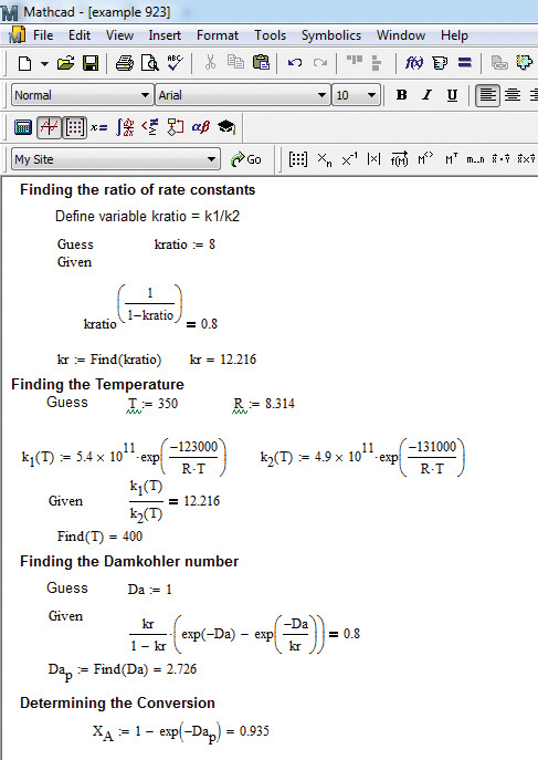
Figure 9.8 Mathcad solution to example 9.2.3.
As can be seen from the figure, the solution involves using a number of solve blocks. The ratio of rate constants is obtained from solving equation E9.6 to be 12.216. This leads to the reaction temperature of 400 K from equation E9.7. The Damköhler number is computed to be 2.726 from equation E9.5, and finally the conversion of A is 0.935 from equation E9.4.
Solution (using Excel)
The solution using Excel involves use of multiple Goal Seek functions. The resulting solution is shown in Figure 9.9.
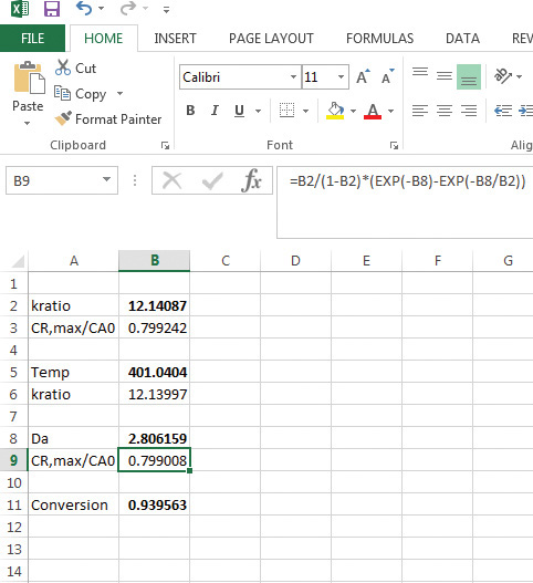
Figure 9.9 Excel solution to example 9.2.3.
It can be seen that both Mathcad and Excel give similar solutions. Excel yields a value of 401 K for the temperature, and the conversion is 0.939. Both these values are very close to the Mathcad solution of 400 K for temperature and 0.935 for conversion.
These three examples offer a glimpse into the nature of computations that a chemical engineer will typically conduct in dealing with topics related to chemical engineering kinetics. Additional practice problems at the end of the chapter provide students with further perspective on these problems.
Leave a Reply