Chemical engineers encounter problems ranging in complexity from simple arithmetic calculations to highly involved ones requiring programming. The following examples present of a few of these problems along with solution techniques using Excel and Mathcad.
EXAMPLE 5.1 FRICTION FACTOR FOR PIPE FLOW
Calculate the Fanning friction factor using the Nikuradse equation for the flow of water through a 1 in. diameter pipe when the Reynolds number is 10,000.
Solution (using a spreadsheet program)
This equation can be solved using a spreadsheet program such as Microsoft Excel. Excel has a built-in function called Goal Seek that enables users to solve the transcendental equation. The stepwise procedure for the solution follows:
1. Enter the Reynolds number value in a cell (B2).
2. Enter an initial guess for the friction factor in another cell (B3).
3. Rearrange equation 5.6 in the form of a function of the Reynolds number and the friction factor (f(Re,f) = 0), as shown below, and evaluate for the values previously entered in another cell (C3).

4. The function value will most likely not equal 0, meaning the initial guess of friction factor was incorrect. Here, an initial guess of 0.1 for the friction factor leads to a function value of –10.44, indicating that the guess was incorrect. Click the DATA tab from the command menu, then the What-if Analysis, and select Goal Seek, as shown in Figure 5.4.4
4. Excel also has a much more powerful Solver utility, which allows a user to manipulate multiple cells, as well as specify constraints on the solution (for example, no negative roots or maximum/minimum solution permitted, etc.) for solving such problems.

Figure 5.4 Goal Seek tool in Excel.
5. This brings up a dialog box, where cell C3 (function) is specified to be set to a value of 0 by manipulating cell B3 (friction factor f), as shown in Figure 5.5. Click OK.
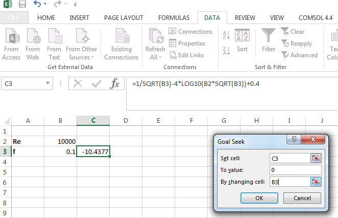
Figure 5.5 Specifying solution constraint in Goal Seek.
Excel reaches a solution by changing the value in the cell B3, ultimately arriving at the f value of 0.0007727, with the function value in cell C3 reaching a value of –5.1E–6 (~0), as shown in Figure 5.6.
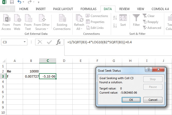
Figure 5.6 Solution of Nikuradse equation by Goal Seek in Excel.
Solution (using Mathcad)
The same problem can also be solved using Mathcad. The stepwise solution procedure is as follows:
1. Specify the value of the Reynolds number by typing Re:10000. (Note that the statement appears as Re := 10000.)
2. Define a function (ff) of Re and friction factor f, by typing the following:
ff(Re,f):4.0*log(Re*\f)-0.40-1/\f
(Note that the asterisk [*] specifies multiplication, the backslash [\] specifies square root, and the forward slash [/] specifies division.)
3. Guess an initial value of f by typing f:0.01.
4. Type f.ans:root(ff(Re,f),f) to use the root command for solution. Typing = at the end of this statement yields 7.727 × 10⁻³ as the friction factor, as shown in Figure 5.7.
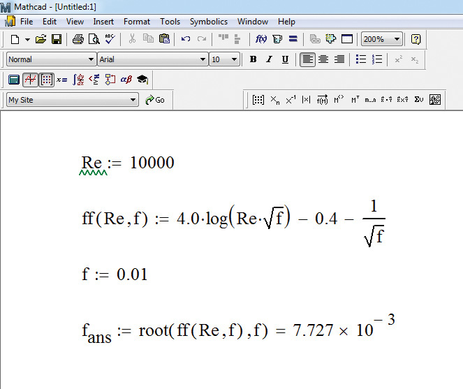
Figure 5.7 Solution of Nikuradse equation using Mathcad.
The appearance of the statements is different from the characters typed. It should also be noted that there are alternative ways to specify the square root in Mathcad. The reader is left to explore the alternatives.
Similar procedures can be used to obtain the solution using other software—MATLAB, Mathematica, Maple, and so on—mentioned previously.
EXAMPLE 5.2 VISCOSITY OF A FLUID
The viscosity of a fluid is a function of temperature and fluid density. The experimentally measured viscosity of water at various temperatures is as shown in Table E5.1. What is the viscosity at 25°C?
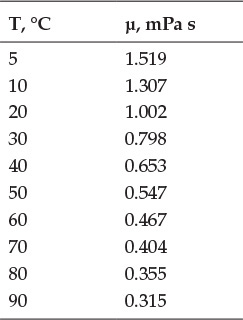
Table E5.1 Water Viscosity as a Function of Temperature
Solution (using a spreadsheet program)
The approach to solving this problem involves fitting a function (polynomial in this case) to the data and evaluating the function at the desired temperature value. The steps involved are as follows:
1. Enter the data from Table E5.1 in two columns.
2. Select the data by clicking in the upper leftmost corner of the data (cell containing number 5) and moving the cursor to the bottom rightmost corner (cell containing the number 0.315) before releasing the button.
3. Click on the INSERT tab on the command menu, and select the scatter plot under the Chart options. This results in an x-y plot being created from the data, as shown in Figure 5.8.
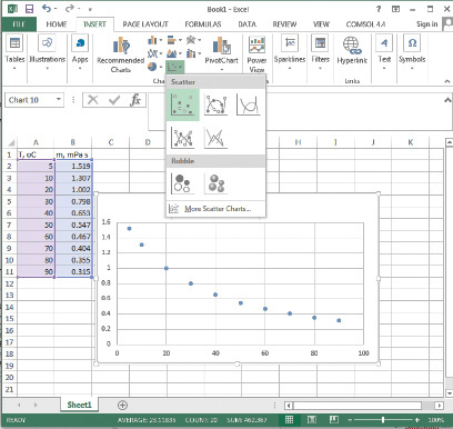
Figure 5.8 Creating a viscosity-temperature plot in Excel.
4. To fit a curve to the data, right-click on a data point to bring up an options box, and select Add Trendline from the menu, as shown in Figure 5.9.
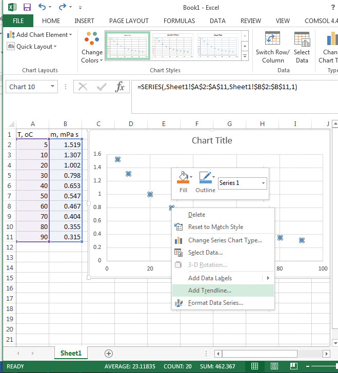
Figure 5.9 Fitting a trendline to the data.
5. A Format Trendline options box opens up to the right of the cells, allowing a number of options for the type of function to be fitted. Select Polynomial of third order (a cubic equation) and check the boxes to obtain the equation and correlation coefficient R2 on the graph. The resulting equation is y = −3e − 6x3 + 0.0006x2 − 0.045x + 1.7154, y being the viscosity and x the temperature. The correlation coefficient for the fit is 0.9993, indicating that a third-order polynomial fits the data accurately within the given temperature range. The resulting graph, the equation of the trendline, and the correlation coefficient are shown in Figure 5.10.
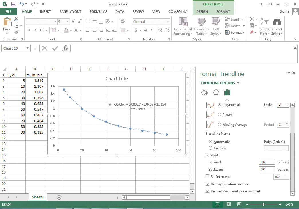
Figure 5.10 Cubic fit of viscosity-temperature data.
6. Evaluate the function at x = 25 to calculate the viscosity at 25°C. This yields a viscosity of 0.9185 mPa s.
Solution (using Mathcad)
The solution using Mathcad starts with creating a data table. The steps are as follows:
1. Click on Insert, and select Data, then Table, from the dropdown menu. This creates a table, whose rows and columns can be populated with the numbers. Insert a table with variable name Temp and another one named μ, entering the temperature and corresponding viscosity values in the first column of the respective tables. (The Greek letter μ is obtained in Mathcad by typing m followed by pressing simultaneously the <Ctrl+g>5 keys.)
5. In this book, Ctrl key combinations are enclosed in angle brackets to indicate that the keys must be pressed simultaneously. For example, <Ctrl+g> means to hold down the Ctrl key and press g.
2. A regress function is used for polynomial regression. The arguments of the function are Temp, μ, and 3, representing the independent variable, dependent variable, and the order of the polynomial, respectively. Type vs:regress(Temp,μ,3)= to obtain a column vector, which consists of the following values: 3, 3, 3, 1.715, −0.045, 5.558 × 10⁻⁴, and −2.556 × 10⁻⁶, as shown in Figure 5.11. The first three numbers represent regress function, location of the first coefficient, and the order of the polynomial, and the last four numbers represent the values of the coefficients in the polynomial starting with the constant. The resulting equation is μ = −2.556e − 6Temp3 + 0.000558Temp2 − 0.045Temp + 1.715, which is close to that obtained using Excel.
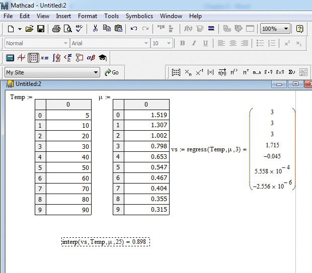
Figure 5.11 Regressing a cubic equation to the viscosity-temperature data in Mathcad.
3. Use the interp function to obtain viscosity at 25°C. This function has four arguments: vs, Temp, μ, and 25; that is, the regression vector, independent variable, dependent variable, and the value of the independent variable at which the function value is desired. Typing interp(vs,Temp,μ,25)= yields a value of 0.898 mPa s for the viscosity.
4. Define a viscosity function using the coefficients previously obtained by typing vis(T):-2.556*10^-6*T^3+5.558*10^-4*T^2-0.045*T+1.715.
5. To create a plot of observed and calculated viscosities, first define a range of temperatures: T:5,5.1;90. Click on the Graph Toolbar button, or choose Insert from the command menu followed by Graph in the dropdown menu, to insert a chart in the program. The resultant graph showing observed data as symbols and calculated values as a line is presented in Figure 5.12. The details of the manipulations are left to the reader.
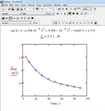
Figure 5.12 Plot of observed and calculated viscosities.
EXAMPLE 5.3 FLOW RATE, AVERAGE VELOCITY, AND REYNOLDS NUMBER
The velocity of a fluid flowing in a circular pipe was measured6 as a function of the radial position and the resultant data are shown in Table E5.2. Calculate the flow rate, average velocity, and Reynolds number if the fluid is water at 25°C. Is the flow laminar?
6. There are several measurement techniques available for measuring the flow rate of a fluid in conduits. Measuring local velocities at various locations in the cross-sectional area for the flow using instruments such as a Pitot tube is one of these techniques.

Table E5.2 Velocity-Radial Position Data
Solution algorithm
The velocity across a cross section of the pipe is assumed to be a function of the radial position only; that is, if one draws a circle having that radius, the velocity is the same everywhere on that circle. In other words, the velocity does not depend on the angular position on that circle. Let v(r) represent the fluid velocity through a thin ring of thickness Δr at radial location r. Then the following gives the flow rate ΔQ through this ring:

Here, 2πrΔr is the area of the circular ring. The schematic representation of the situation is shown in Figure 5.13.
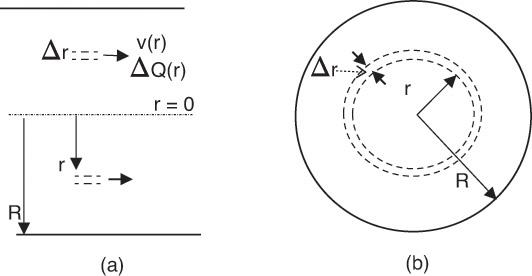
Figure 5.13 Flow through pipe—(a) side view, (b) cross-sectional view.
The total flow rate is simply the summation of all such flow rates calculated at the locations where the velocity is measured:

When the thickness of the ring becomes vanishingly small, equation E5.3 turns into an integral:

The average velocity and Reynolds number are calculated from equations E5.5 and E5.6, respectively.


Here, D is the pipe diameter, ρ the density, and μ the viscosity of the fluid.
Solution (using a spreadsheet program)
The calculations using Excel are shown in Figure 5.14.
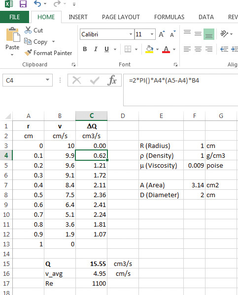
Figure 5.14 Excel solution to Example 5.3.
As seen from the figure, data from Table E5.2 are entered in columns A and B, and the flow rate at various locations is calculated in column C. The calculation for cell C4 can be seen in the figure, the formula entered by typing =2*pi()*A4*(A5-A4)*B4, corresponding to the terms in equation E5.2. The total flow rate is obtained by summing the flow rates in cells C3 through C12 by typing the formula =Sum(C3..C12) in cell C15. As seen from the figure, the total flow rate is calculated to be 15.55 cm3/s. The average velocity is calculated by entering =C15/F7 in cell C16, and the Reynolds number by typing = C16*F8*F4/F5 in cell C17. The parameter values of the radius of the pipe, density, and viscosity are entered in cells F3, F4, and F5. The cross-sectional area is calculated in cell F7 (=pi()*F3^2), and cell F8 contains the diameter of the pipe, which is twice the radius (=2*F3). The average velocity is 4.95 cm/s, and the Reynolds number is 1100, indicating that the flow is laminar.
Solution (using Mathcad)
The solution using Mathcad is shown in Figure 5.15, and the calculation steps follow.
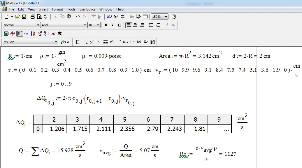
Figure 5.15 Mathcad Solution to Example 5.3.
1. Enter the parameters radius, density, and viscosity as follows: R:1*cm, r<Ctrl+g>:1*gm/cm^3, and m<Ctrl+g>:0.009*poise, respectively. (As mentioned previously, pressing <Ctrl+g> after a Roman script letter changes it to a Greek symbol.) Enter the units using multiplication/division operations. The appearance of the parameters and variables can be seen in the figure.
2. Calculate the cross-sectional area and diameter by entering A:p<Ctrl+g>*R^2 and d:2*R, respectively. Typing the = sign after entering these formulae yields the values of the area and the diameter. Mathcad automatically assigns SI units to quantities, yielding area in square meters (m2) and diameter in meters. The units are changed to square centimeters (cm2) and centimeters by clicking on the Mathcad units and entering the desired units.
3. Enter the radial position and velocity data by defining row matrices for each: r:<Ctrl+m> and v.r:<Ctrl+m>. The <Ctrl+m> key sequence brings up an Insert Matrix dialog box; enter the number of rows (1) and the number of columns (11). Click OK in the dialog box to create the matrix, and enter the respective data values. Assign units to the variables r and vr in a similar manner as earlier; that is, using multiplication/division operations. (It should be noted that typing v.r creates a variable named vr. The subscript r is not the index of the variable.)
4. Calculate the flow rate in each ring (corresponding to equation 5.7) by entering D<Ctrl+g>Q.r[0,j:2*p<Ctrl+g>*r[0,j *(r[0,j+1 -r[0,j)*v.r[0,j. (Note that three spaces must be inserted after “j+1” and two spaces must be inserted between “j” and “)” in this expression.) The key sequence D<Ctrl+g>Q.r creates the variable ΔQr, and the sequence [0,j identifies it as the flow rate corresponding to the jth location. Of the terms on the right side of the equation, r[0,j represents the radial location r, (r[0,j+1 -r[0,j) represents the thickness of the ring, and v.r[0,j represents the velocity corresponding to that radial location. As seen from Figure 5.14, ΔQr is a matrix containing 1 row and 10 columns, with the numbers representing the flow in each differential element. The range of index j needs to be defined before these flow rate calculations can be performed; type j:0;9. To obtain the total flow rate Q by summation of the ΔQr values, type Q:<Ctrl+4>D<Ctrl+g>Q.r. The <Ctrl+4> sequence inserts the summation operator in the Mathcad worksheet.
5. Calculate the average velocity and the Reynolds number by entering the appropriate formulae. As mentioned previously, the units by default are SI units and need to be changed if the answers are desired in other units.
It can be seen that the solution using Mathcad differs slightly from that obtained using Excel. The explanation for this discrepancy is left to the reader.
EXAMPLE 5.4 SHEAR FORCE ON PIPE WALL
For the flow problem in Example 5.3, what is the shear force exerted at the pipe surface? Assume the pipe length to be 2 m.
Solution algorithm
The shear force, Fshear, is obtained by multiplying the shear stress by the area of the surface (Ashear) over which it acts. From equation 5.2, we get the following:

Here Ashear is given by the following:

The velocity gradient is obtained from the data in Table 5.2. The following is used for numerical differentiation:

Solution (using a spreadsheet program)
The calculations using Excel are shown in Figure 5.16.
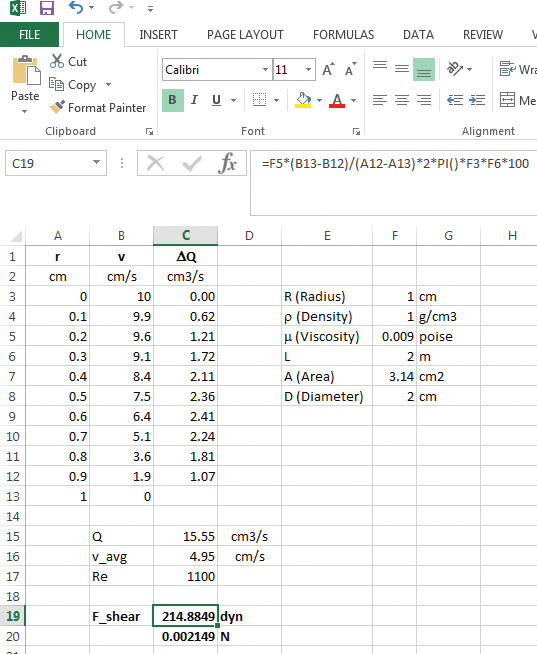
Figure 5.16 Shear force calculation using Excel.
The length of pipe is shown in cell F6. The shear force calculation is in cell C19 with the formula as shown. The conversion factor of 100 is used to convert the length units from meter to centimeter. The shear force obtained is ~214 dyn. The answer unit is converted into SI unit force (newtons, or N) using a conversion factor of 1 dyn = 10−5 N.
Solution (using Mathcad)
The solution involves inserting the following statements in the previous Mathcad document:
1. L:2*m
2. F.shear:m<Ctrl+g>*(v.r[0,10 -v.r[0,9)/r[0,9 -r[0,10 *2*p<Ctrl+g>*R*L
(Note that two spaces are inserted before “-v.r”; one space before “)”; one space before “-r”; and four spaces before “*2*”.)
The shear force is calculated to be 2.149 × 10⁻³ N, as seen in Figure 5.17.
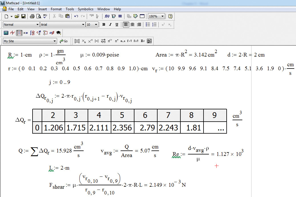
Figure 5.17 Shear force calculation using Mathcad.
The result is identical to that obtained using Excel. Entering the formula in Excel is slightly easier than in Mathcad. On the other hand, Mathcad offers automatic conversion of units, removing the need for manually entering the conversion factors.
The accuracy of derivative computations increases with a decrease in the thickness of the ring. Additional radial position-velocity data availability at intervals of 0.05 cm rather than 0.1 cm would increase the number of computations but enable us to estimate the velocity derivative more accurately. The flow rate computations would also be more accurate.
Leave a Reply